Interval arithmetic uses worst case estimates to get an inclusion for results. This can be essential, if the source data are already not precisely known. But even if they are, the computation may spoil the result. Interval arithmetic uses fixpoint theorems to guarantee that there is a solution in the computed interval.
This notebook introduces the interval arithmetic of Euler. For a reference to intervals and algorithms using intervals have a look at the following pages.
The closed interval [2,3] is entered with the following notation.
>~2,3~
~2,3~
Alternatively, you can use plus-minus. If you do not have this key, press F8.
>2.5±0.1
~2.4,2.6~
Plus-Minus is also available for output.
>ipmprint(2±0.1)
2±0.1
To set this output format permanently, use ipmformat. To reset to the normal format, call ipmformat(false).
>ipmformat(true); ~1,2~, ipmformat(false);
1.5±0.5
Operators between intervals yield an interval result.
The basic rule is: The result contains all possible results, when the operator is applied to all arguments in all intervals.
>~2,3~ * ~4,7~
~8,21~
Note that the following two expressions are different.
>~-1,1~^2, ~-1,1~*~-1,1~,
~0,1~
~-1,1~
The first one contains all squares of elements in [-1,1], the second contains all s*t, where -1 <= s,t <=1.
The interval ~s~ is a small interval around s.
>~2,2~, ~2~,
~2,2~
~1.9999999999999996,2.0000000000000004~
For a simple example, we compute the height of a mountain in 20.2km distance, which appears at an angle of 3.2° above the current level. We assume that all values are known to the significant digits.
>d=20.2km±0.05km; a=3.2°±0.05°; d*sin(a)
~1107,1149~
Indeed, if we take the extremal values of our errors, we get a large interval of possible results.
>20.15km*sin(3.15°), 20.25km*sin(3.25°),
1107.24612524
1148.02894816
Evaluating a longer expression in the interval arithmetic can lead to error propagation. Assume we have the following function.
>expr="x^3-x^2-2*x";
Let us evaluate the function in an interval of length 0.2.
>x:=1.2±0.1; expr(x)
~-3,-1.2~
As we will see, this is not a good inclusion of the result. One of the main reasons is, that the interval evaluation takes a different x from the interval, whenever the variable x occurs, and includes all these results.
The function "mximieval" uses Maxima to compute the derivative of the expression, and with the derivative, we get a much closer inclusion.
>mxmieval(expr,x)
~-2.3,-2~
Sub-dividing the interval yields an even better inclusion.
>mxmieval(expr,x,20)
~-2.12,-2.07~
A simple subdivision may lead better results too, but with more effort. However, we do not have to compute the derivative. So this method works for functions too, not only for expressions.
>ieval(expr,x,100)
~-2.13,-2.07~
If we plot the function, we see, that the maximal value on the interval is at 1.1, and the minimal value is somewhere inside the interval.
>plot2d(expr,1.1,1.3):
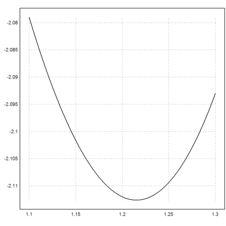
We can find the place of the minimum with fmin, and then evaluate the expression there to get the minimal value. Thus we get the true limits of the image of [1.1,1.3] under this mapping.
>expr(fmin(expr,1.1,1.3)), expr(1.1)
-2.11261179092
-2.079
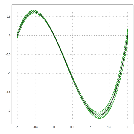
We can make a plot of an interval function. To demonstrate this, we disturb the x values -1 to 2 by 0.01, and evaluate our expression. We print the first three values only.
>x:=-1:0.01:2; y:=expr(x±0.01); y[1:3]
[ ~-0.07,0.07~, ~-0.04,0.098~, ~-0.01,0.13~ ]
The plot2d function will plot the y-ranges as a filled curve.
>plot2d(x,y,style="\/"); plot2d(x,expr(x),thickness=2,add=1):
The 10-th partial sum of the Taylor series of exp is the following polynomial.
>p=1/fac(0:10); fracprint(p')
        1
        1
      1/2
      1/6
     1/24
    1/120
    1/720
   1/5040
  1/40320
 1/362880
1/3628800
Check with Maxima.
>&taylor(exp(x),x,0,10)
          10        9       8       7     6     5     4    3    2
         x         x       x       x     x     x     x    x    x
       ------- + ------ + ----- + ---- + --- + --- + -- + -- + -- + x
       3628800   362880   40320   5040   720   120   24   6    2
                                                                   + 1
We evaluate this polynomial in -2.
>longformat; evalpoly(-2,p)
0.135379188713
Compare to the correct result for the infinite series.
>exp(-2)
0.135335283237
We can get an inclusion of the true value from the Taylor expansion with the remainder term in interval notation. The error of the series expansion is less or equal the next term in the series, since the series is alternating.
Note that we have to use ~p~ because p is not exactly represented in the computer. But we can use the one point interval [-2,-2].
>evalpoly(~-2,-2~,~p~)+~-1,1~*2^11/11!
~0.13532,0.13544~
Some more terms. Note that 21! is exactly representable in the computer.
>n=20; evalpoly(-2,~1/fac(0:n)~)+~-1,1~*2^(n+1)/fac(n+1)
~0.135335283236606,0.135335283236695~
The interval arithmetic provides guaranteed inclusions of zeros of functions using the interval Newton method.
For this, we need a function f and its derivative f1.
>inewton("cos(x)-x","-sin(x)-1",1)
~0.73908513321516045,0.73908513321516089~
Maxima can compute the derivative for us.
>mxminewton("cos(x)-x",~0,1~)
~0.73908513321516045,0.73908513321516078~
Compare with the real Newton method.
>longestformat; newton("cos(x)-x","-sin(x)-1",1)
0.7390851332151607
There is a very simple function, which uses a bisection method controlled by interval computation.
>ibisect("cos(x)-x",0,1)
~0.7390851332139,0.7390851332154~
One famous example occurs, if we imagine a chord around the earth, which is 1m longer than the perimeter of the earth. We lift that chord at one point. How high can we lift it?
If we denote the angle of lifting by 2*alpha, the problem is essentially equivalent to the solution of
![]()
Let us try this.
>r=rEarth$; alpha=bisect("tan(x)-x",0,0.1,y=1/(2*r))
0.006179449475166621
From this, we get the height with elementary trigonometric computations.
>r*(sec(alpha)-1)
121.3701123662059
We have no idea, how good this solution is. So we check with an interval solver, and find that the answer is quite reliable.
>mxminewton("tan(x)-x",alpha,y=1/(2*r)); r*(sec(%)-1)
~121.37011238,121.370112386~
For larger values of r, we get less reliable results.
>r=1.2e15; ibisect("tan(x)-x",0,0.1,y=1/(2*r)); r*(sec(%)-1)
~69622.9,69624.9~
Let us try a multidimensional example. We solve
![]()
First, we need a function.
>function f([x,y]) &= [x^2+y^2-1,x^2/2+2*y^2-1]
                                           2
                       2    2         2   x
                     [y  + x  - 1, 2 y  + -- - 1]
                                          2
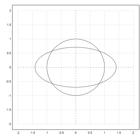
First we plot the contour lines of the first and the second component of f, i.e., the solutions of f_1(v)=0 and f_2(v)=0. The intersections of these contour lines are the solutions of f(v)=0.
>plot2d("x^2+y^2",r=2,level=1); ...
 plot2d("x^2/2+2*y^2",level=1,add=1):
For the Newton method, we need a derivative matrix.
>function df([x,y]) &= jacobian(f(x,y),[x,y])
                             [ 2 x  2 y ]
                             [          ]
                             [  x   4 y ]
Now we are ready to get an inclusion of the intersection points (the zeros of f) using the two dimensional Newton method. The interval Newton method yields a guaranteed inclusion of one of the solutions.
>inewton2("f","df",[~0.8,0.9~,~0.5,0.6~])
[ ~0.8164965809277252,0.816496580927727~,
~0.5773502691896251,0.5773502691896264~ ]
The usual Newton method yields the solution as a limit point of the Newton iteration.
>newton2("f","df",[1,1])
[0.816496580927726, 0.5773502691896257]
The Broyden method does the same, but does not deliver a guaranteed inclusion. It does not need the derivative.
>broyden("f",[1,1])
[0.816496580927726, 0.5773502691896257]
There are also interval solvers for differential equations. We try
![]()
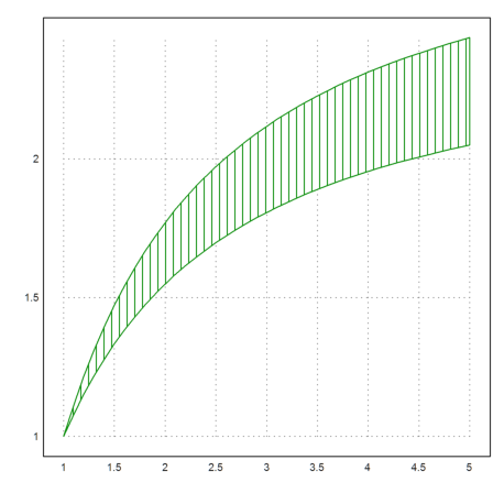
The first, very simple interval solver does not use derivatives and is very coarse. We get a very rough inclusion with the step size 0.1.
>x=1:0.1:5; y=idgl("y/x^2",x,1); plot2d(x,y,style="|"):
With a finer step size of 0.01, the inclusion is better.
>x=1:0.01:5; y=idgl("y/x^2",x,1); plot2d(x,y,style="|"):
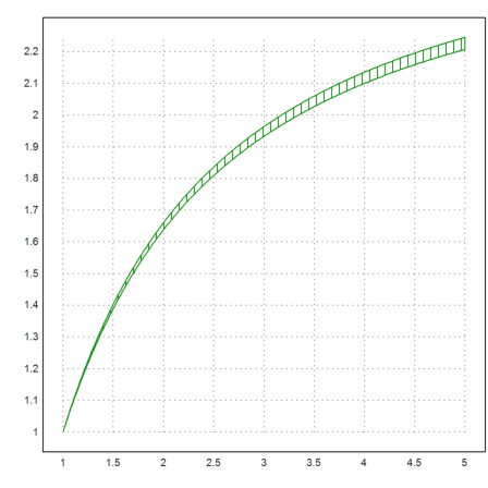
The following solver uses a high order method and Maxima. We get a very good inclusion.
>y=mxmidgl("y/x^2",x,1); y[-1], plot2d(x,left(y)_right(y));
~2.225540928492,2.2255409284929~
Of course, the default ode solver gets a good result too, and very quickly.
>ode("y/x^2",1:0.1:5,1)[-1]
2.225540928476129
Let us demonstrate the use of interval methods for the inclusion of a Eigenvalue.
We first generate a random postive definite matrix.
>A=random(20,20); A=A'.A;
Then we compute its Eigenvalues in the usual way.
>l=sort(re(eigenvalues(A)));
We take the first Eigenvalue.
>longformat; l=l[1]
1.23982900772e-006
Compute an eigenvector.
>x=eigenspace(A,l);
We normalize it in a special way.
>x=x/x[1];
We now set up the function
![]()
with
![]()
>function f(x,A) ...
 n=cols(x); return ((A-x[1]*id(n)).(1|x[2:n])')';
 endfunction
The following is the starting point of our algorithm.
>lx=l_x[2:cols(A)];
We could use the Broyden method to determine the zero of this function.
>yb=broyden("f",lx';A); yb[1],
1.23982900752e-006
For the interval Newton method, we define the Jacobian of f.

>function f1(x,A) ...
 n=cols(x);
 B=A-x[1]*id(n);
 B[:,1]=-(1|x[2:n])';
 return B;
 endfunction
Let us expand lx a bit, so that it probably contains a solution of f(x)=0.
>ilx=expand(~lx~,1000000000);
The interval Newton method now proves a guaranteed inclusion of the Eigenvalue.
>{y,v}=inewton2("f","f1",ilx';A); y[1]
~1.239828965e-006,1.239829051e-006~
v=1 means, that the inclusion is verified.
>v
1
We try to compute
![]()
1/n is much smaller than 1, and while 1+1/n is correct up to 16 digits, we loose many digits from 1/n.
>longestformat; n=12346789123; 1+1/n
1.000000000080993
And thus the following result is inaccurate, if we compare to the correct result. This is called cancellation.
>(1+2/n)-(1+1/n), 1/n
8.09927680478495e-011
8.099271721885713e-011
Using interval arithmetic, we can see that our result is not good.
>(1+2/~n~)-(1+1/~n~)
~8.099232e-011,8.099322e-011~
As a consequence, the following approximation of E is much worse than it should be.
>(1+1/n)^n, E
2.718283534274811
2.718281828459045
The correct error is of the order E/n~=1e-10. But we have only 1e-6. We can compare with a slow long precision computation in Maxima.
>&fpprec:30; &:float((1+1b0/@n)^@n) // (1+1/n)^n with 30 digits
2.718281828348965
However, with a binomial expansion and an estimate we get a much more precise evaluation of (1+1/n)^n.
>kn:=15; k=~1:kn~; 2+sum(cumprod((1-k/n)/k)/(k+1))+~0,1/kn!~
~2.7182818283489,2.7182818283498~
We can design a function for log(1+x), which works even for very small x. Depending on the size of x, we use a Taylor expansion for log(1+x), or the usual evaluation. The Taylor expansion can be computed by Maxima at compile time.
>function map logh (x:scalar) ...
   ## Compute log(1+x) exactly
   if abs(x)<0.001 then
     res=&:taylor(log(1+x),x,0,7);
     if isinterval(res) then
       res=res+~-0.001^8/(8*0.999^8),0~;
     endif;
     return res;
   else
     return log(1+x);
   endif;
 endfunction
Now we get a good evaluation of (1+1/n)^n.
>exp(n*logh(1/n))
2.718281828348965
And for intervals we get an exact inclusion of the value.
>exp(n*logh(1/~n~))
~2.71828182834895,2.71828182834897~